Subsea SLAM EKF Simulation

Noel Zinn, www.hydrometronics.com, August 2018

Simultaneous Location and Mapping (SLAM) is an observational and mathematical technique that enables walking, rolling, sailing or swimming robots to navigate indoors (or in a park with trees, or anywhere for that matter ... just not in a desert or a seafloor with no topography) without any external (absolute) positioning aid such as GPS, USBL or LBL. First, a robot entering the environment at nominal (0,0) or estimated coordinates scans the environment. Scanning instruments might be sonar (like a bat), or LIDAR (similar principle but with coherent light), for example, or even a real-time camera, but cameras present special analysis challenges. Then the scans must be analyzed (rather quickly) for anomalies that might be landmarks, such as a discontinuity or "spike" between samples indicating a tree (perhaps) standing out from its background or a trend reversal that might be the corner of two orthogonal walls. We presume a few things about the robot. First, the robot knows its orientation just like a boy scout always knows north, either with a magnetic compass (marginal technology) or a sensitive, north-seeking IMU. Second, the robot knows the ranges and/or the bearings (angles relative to its north) to the landmarks that it identifies (SLAM can use ranges or bearings or both).  This is straightforward with sonar and LIDAR but challenging with a camera, which may require different perspectives ... thus odometry. Third, the robot knows its odometry, that is, how far and in which direction it travels. At the robot's next location (called a "pose" in the SLAM literature), it scans again and identifies old (and maybe new) landmarks. Now a new challenge arises. The robot must associate ... or not ... the landmarks of the second scan with the landmarks of the first scan. With good odometry and good ranges and bearings to the landmarks, this is possible. 

All of the preceding (scanning, identification and association) is very much sensor specific and involves special software techniques. Bravo to those who can do it. These are the observational techniques of SLAM, which are very difficult to program in the abstract. One needs to purchase some hobby boards from Seeed or Adafruit to work at this level (maybe another paper) ... or have a large budget (I don't). OTOH, scanning, identification and association can be simulated in just a few lines of code. After the observational techniques of SLAM comes a more interesting challenge (for me), the mathematical techniques of SLAM. What to do with the associated landmarks and the odometry? Where is the robot? Where are the landmarks? Answers are generally provided by an Extended Kalman Filter (EKF), although there are other solutions to this problem. A Kalman filter is a linear algorithm that weighs the relative merits of observations (scanning) and transition (odometry) and decides the optimal ratio (called the Kalman gain) to be applied. Rudolf Kalman was an electrical engineer and applied to electrical problems (e.g. scalar measurements of voltage and amperage) the Kalman filter is, indeed, linear. But applied to ranges and bearing, which are non-linear, modification is required. Thus the EKF.  The "extension" of the EKF is to linearize the range and bearing observation equations by preserving the first-order terms of a Taylor's series expansion in what's called a Jacobian matrix (or vector) of partial differentials. So, an EKF is just a Kalman filter with linearized observations.  

Here's how it works. From the first scan, identification and association steps of the observational techniques of SLAM, we preserve the robot pose and the ranges and bearings to the identified landmarks (which we number for convenience). This information is sufficient (with a little trigonometry) to assign coordinates to the identified landmarks. Then the robot moves. From the second and subsequent scan-identification-association steps we again preserve the robot poses and the observations. From these later poses we can predict the ranges and bearings to the landmarks even before they are observed. The predicted minus the observed (P-O) is called an innovation. In a Kalman filter the innovation has a role similar to that of the residual (C-O, computed minus observed) in least-squares estimation. This iterative process (scan, travel, scan) comprises the deterministic model of a Kalman filter.

The stochastic (or statistical) model of a Kalman filter accommodates the uncertainties (errors, probabilities) of robot and landmark positions. A Kalman filter runs on odometry and observations and no odometry or observation is perfect. Each has error ... and nowadays the euphemistic way to say "error" is "uncertainty". The quality of the robot's north reference has error as does the distance travelled forward. Observed ranges and bearings have error ... to say nothing about correct landmark association without which all else fails. In a Kalman filter all these uncertainties are assumed to be normal or Gaussian, that is, distributed like a bell curve. And then there's time. The longer a robot travels without scanning and updating its position, the more error it accumulates. As noted previously, the job of a Kalman filter is to arbitrate among all this uncertainty. The mathematical steps are these: (1) to transition forward (odometry) while updating position (the "state" vector) and increasing ("blooming") state uncertainty (the "P" matrix) as a consequence of odometry (transition), (2) to predict the observations to the landmarks, linearize them into the Jacobian (H) vector, and, given P and the observational uncertainty ("R"), compute the Kalman gain ("K"), (3) to compute the innovations, to multiply them by K, and to update the state, (4) to use K, H and P to decrease ("groom") P (the state uncertainty matrix) as a result of the new observations, and (5) to transition forward again and repeat the steps. The matrix algebra of each step is just a single line of code in Matlab. It's worth noting that, in 2-D SLAM, the state vector contains the X and Y positions of the robot, but also its orientation w.r.t. north (called theta), plus the X and Y positions of all the landmarks. (3-D SLAM is a simple extension of this into the vertical dimension.) Consequently, the state vector and especially the P matrix (of size state vector squared) can be very large and slow to process. FastSLAM (not addressed in this paper) is a method of particulating the problem for faster computation. As the process runs, the robot and the landmarks become highly correlated in the P matrix. That's another way of saying that the landmarks and the robot become one, relative entity, truly Simultaneous Location and Mapping (SLAM).  

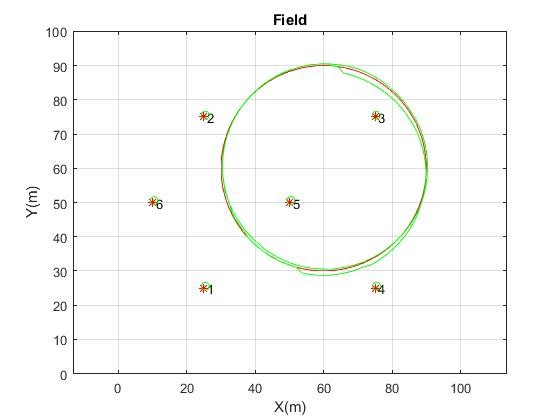
Having disposed of these preliminaries, the simulation to be discussed is that in the first graphic titled "Field" containing six numbered landmarks and the circular path of an autonomous underwater vehicle (AUV). The landmarks may be the edges of PLETs, PLEMs, or risers in a subsea installation. The AUV observes landmarks within range (30 meters in this simulation) while making two loops, the first to close the loop and the second to benefit from the correlations induced by loop closure. The red path and the red landmarks are the simulated truth; the green path and the green landmarks are where the SLAM EKF "thinks" things are. The AUV enters the field with an uncertainty of 2 meters (accumulated, perhaps, during descent). The landmarks are assigned an uncertainty of 4 meters because they are initially determined by an uncertain AUV with uncertain observations, later to be updated by SLAM. Subsea LIDAR range uncertainty is 0.2 meters and bearing uncertainty 0.2 degrees relative to an uncertain robot orientation. The AUV has an IMU onboard with a course uncertainty of 1% and an azimuth uncertainty of 0.5 degrees. It may or may not be DVL aided, but it certainly is not USBL or LBL aided, that is, there are no absolute positioning sensors. The AUV travels around the circle in steps of 4 degrees in this simulation. 

The second plot titled "Theta w.r.t. to true azimuth" is a plot of the third element of the state vector, the orientation of the AUV minus the true simulated azimuth. We should expect something close to zero degrees. Notice that the plot is a bit ragged during the first rotation through the field, but that it settles down nicely during the second rotation after loop closure. The third plot titled "AUV dX in blue, dY in green" shows the difference between the EKF path of the AUV and the true simulated path. These differences are, of course, due to the random errors in the system. The algorithm makes ample use of Matlab's random number generator to perturb the true odometry and the true observations. Run the simulation again and you get different plots, but these are typical and within the expectations of the EKF itself as contained in the final P matrix (state vector uncertainties). P-matrix positional standard deviations are 1.3 meters. The "AUV dX in blue, dY in green" plot is showing differences of about 0.5 meters in each axis, well within P-matrix expectations. The fourth and final plot "Landmark offsets from true" shows that the EKF positions of all six landmarks are tightly grouped about 0.4 meters from true in X and about 0.5 meters from true in Y. This is consistent with the previous plot "AUV dX in blue, dY in green". So, as a result of two rotations of the AUV through the field we have a map of the field with the AUV posed within it that is about half a meter different from the simulated truth in X and Y, a difference that is consistent with the expectations of the EKF. And now the AUV can continue to swim indefinitely within the field without absolute positioning sensors (USBL or LBL) while maintaining this level of accuracy. In fact, the landmarks are now playing the role of LBL beacons, whereas they were completely uncoordinated at the beginning of the SLAM process. Is SLAM perfect? No. Is any positioning sensor (absolute or otherwise) perfect? No. But SLAM does a pretty good job in the absence of USBL and LBL, which are expensive and time consuming to deploy and maintain. SLAM sails right up to the field and gets to work.